This tutorial is built upon efforts of Mo Heydarian and Mallory Freeberg and tools wrapped by Björn Grüning, Marius van den Beek and other IUC members.

Introduction

We will use RNA-seq data from a study published by Wu et al. in 2014 DOI:10.1101/gr.164830.113. The goal of this study was to investigate "the dynamics of occupancy and the role in gene regulation of the transcription factor Tal1, a critical regulator of hematopoiesis, at multiple stages of hematopoietic differentiation." To this end, RNA-seq libraries were constructed from multiple mouse cell types including G1E - a GATA-null immortalized cell line derived from targeted disruption of GATA-1 in mouse embryonic stem cells - and megakaryocytes. This RNA-seq data was used to determine differential gene expression between G1E and megakaryocytes and later correlated with Tal1 occupancy. This dataset (GEO Accession: GSE51338) consists of biological replicate, paired-end, poly(A) selected, stranded (dUTP) RNA-seq libraries. Because of the long processing time for the large original files, we have down-sampled the original raw data files to include only reads that align to chromosome 19 and a subset of interesting genomic loci identified by Wu et al.

Key fact about this study:

• TAL1 is a transcription factor essential for hematopoesis. It is critically needed for establishing hematopoetic stem cells during embryonic development and to differentiate between erythroid and myeloid cell lineages, including those leading to megakaryocytes, mast cells, and eosinophils.
• Some of the TAL1 molecules are components of multiprotein complexes that also include other transcriptional factors such as GATA-1.
• By contrasting RNA from GATA-null G1E cells with that of megakaryocytes we can identify transcripts regulated by GATA-1 dependent TAL1.

Schematic representation of hematopoesis (from Wikipedia)

Analysis strategy

The goal of this exercise is to:

1. Identify what transcripts are present in the G1E and megakaryocyte cellular states
2. Which transcripts are differentially expressed between the two states.

We will use a de novo transcript reconstruction strategy (not to be confused with the de novo RNAseq when reference genome is not known) to infer transcript structures from the mapped reads in the absence of the actual annotated transcript structures. This will allow us to identify novel transcripts and novel isoforms of known transcripts, as well as identify differentially expressed transcripts.

Tutorial Agenda

In this tutorial, we will address:

1. Data upload
2. Read QC and pre-processing
3. Read mapping
4. De novo transcript reconstruction
5. Transcriptome assembly
6. Read counting and differential expression analysis
7. Visualization

The Data

Due to the large size of this dataset, we have down-sampled it to only include reads mapping to chromosome 19 and certain loci with relevance to hematopoeisis. This data is available from two sources:

• Zenodo (use these data on any Galaxy instance)
• Galaxy data library (use these data on main Galaxy server at http://usegalaxy.org).

Data organization and naming

The data is structured in the following way:

• There are two samples: G1E cells and megakaryocytes (G1E and Mk)
• There are two biological replicates per sample: R1 and R2
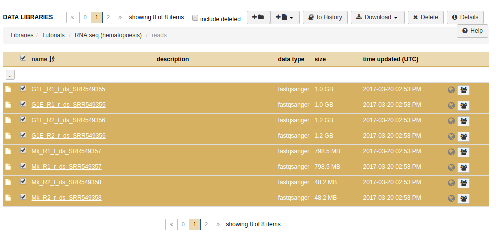
• Each replicate has forward and reverse reads (f and r)
• Thus, there are eight (8) fastq files

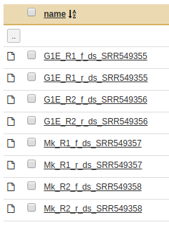Galaxy data library containing the reads. Here you can see two cell types (G1E and Mk) with two replicates for each cell type (R1 and R2). Each replicate is requested with paired-end reads (f and r).

How to upload the data into Galaxy

Once you upload data into a new history you Galaxy interface should look like this:

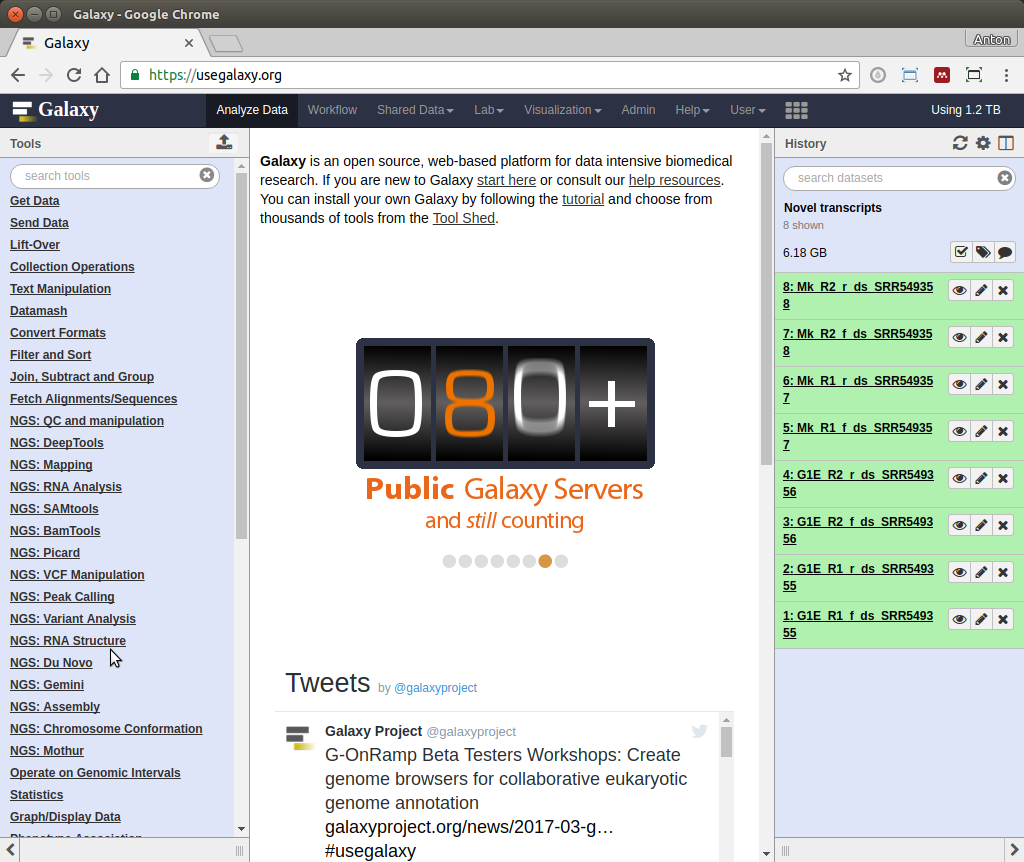Datasets are uploaded into a new history. Here the history was named Novel transcripts. You can name history as well by clicking on its name. For more info on histories see this tutorial.

Exploring the data

To lean more about the data we will be using let's look at just one set of reads. This will give us an idea on how good the data is and what we might need to do with it before proceeding with the analysis.

Assess data quality

For quality control, we use similar tools as described in NGS-QC tutorial: FastQC and Trimmomatic.

Let's start by processing the smaller set of reads from G1E set: G1E_R1_f_ds_SRR549355 and its reverse set of mates G1E_R1_r_ds_SRR549355 using NGS: QC and manipulation -> FastQC:

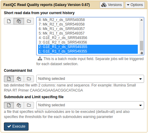QC'ing reads with FastQC. Note we've pressed the button to enable selection of multiple datasets within the Short read data from your current history box.

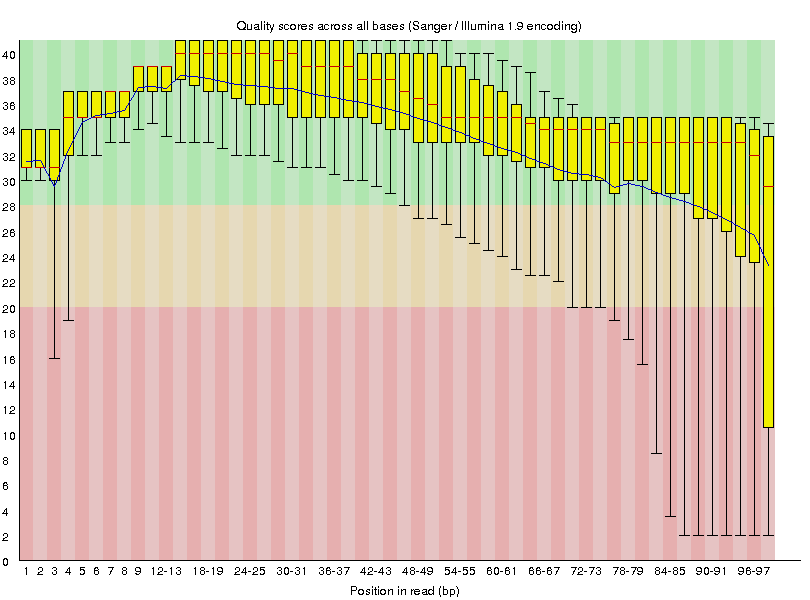
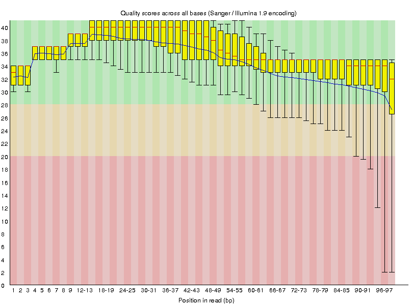
This will generate the following quality value distributions:

G1E_R1_f_ds_SRR549355	G1E_R1_r_ds_SRR549355

Dynamically trim low quality bases from reads' 3' ends

The quality score distributions we seen above for one sample are characteristic of all reads in our dataset (you can run FastQC on remaining reads to see if this is true). To increase mapping efficiency we can trim off the low quality bases from the ends of the reads using NGS: QC and manipulation -> Trimmomatic:

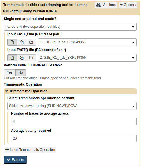Running trimmomatic on G1E_R1 read pair.

Trimmomatic will produce four outputs as a result:

• Trimmomatic on G1E_R1_f_ds_SRR549355 (R1 paired)
• Trimmomatic on G1E_R1_f_ds_SRR549355 (R2 paired)
• Trimmomatic on G1E_R1_f_ds_SRR549355 (R1 unpaired)
• Trimmomatic on G1E_R1_f_ds_SRR549355 (R2 uppaired)

The unpaired datasets we will no longer need in our analysis.

Now that we've ran trimmomatic let's see if it had any effect on our data. We can do this by rerunning FastQC on G1E_R1_f_ds_SRR549355 and G1E_R1_r_ds_SRR549355 datasets after they have been trimmed. This will generate the following quality value distributions:

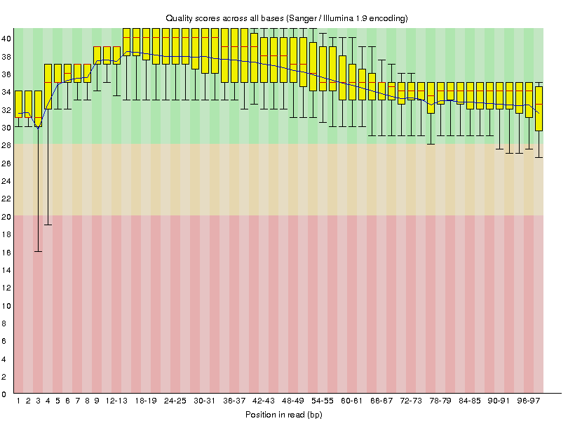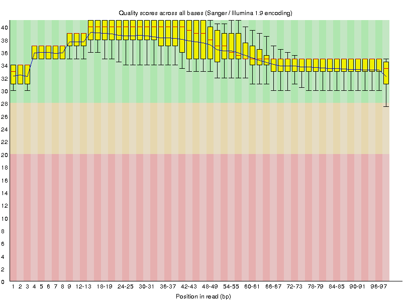G1E_R1_f_ds_SRR549355	G1E_R1_r_ds_SRR549355

Is this a stranded RNAseq experiment?

RNAseq data is often stranded as it significantly increases its utility. But how do you know you have a stranded data? Moreover, if data is indeed stranded is it derived from first or second cDNA strand? To answer this question we can map the data and analyze mapping properties. Let's do that on the same set of forward and reverse G1E_R1 datasets.

Map subset of data

Here we will use NGS: RNA analysis -> HISAT to map the reads against the mouse genome:

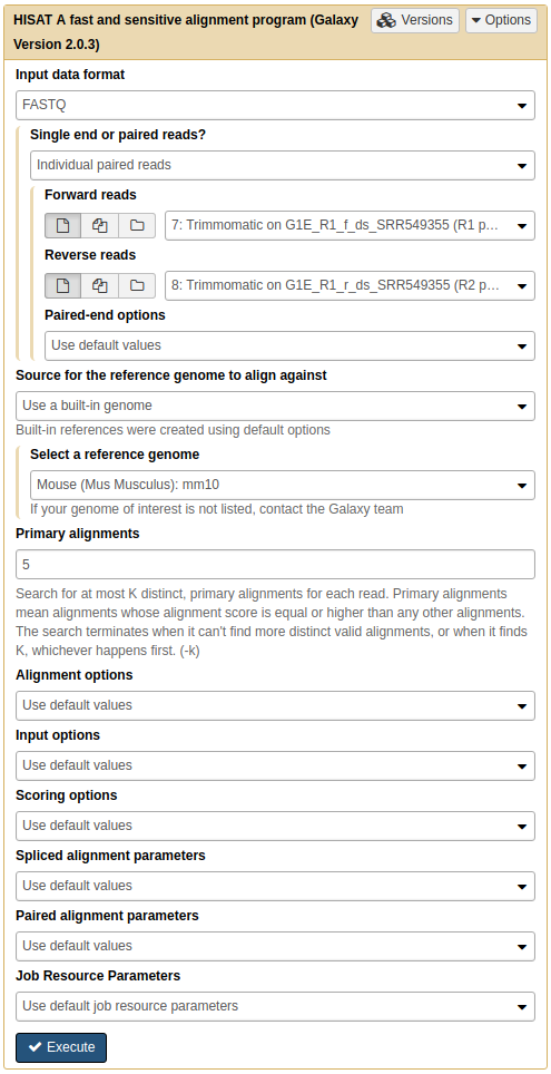Running HISAT with default parameters on trimmed data. Select Individual paired reads from Single or paired reads? dropdown to be able to select individual fastq datasets. Make sure you select correct inputs (do not select unpaired trimmomatic outputs by accident).

Filter and restrict to a small region of interest

All we need is to look at read mapping around some known gene (pick any well expressed gene you like). To do this we will filter BAM dataset using NGS: SAMtools -> Filter SAM or BAM:

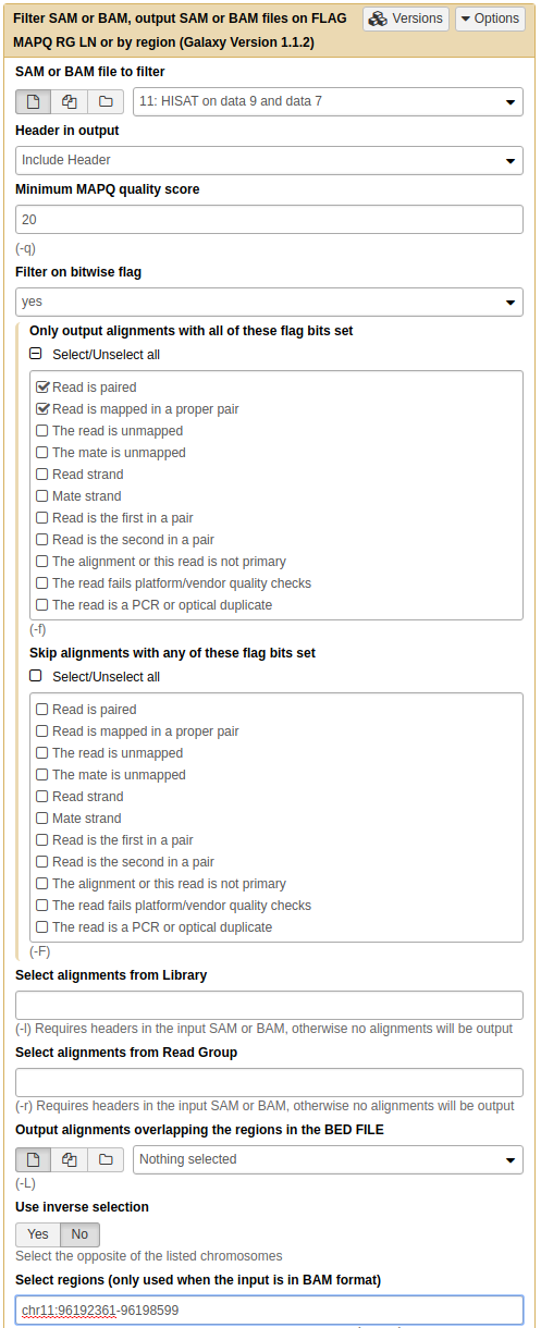|Filter BAM data to retain only well mapped reads (Minimum MAPQ quality score is 20) that are in proper pairs and mapped around position chr11:96192361-96198599.

Display at IGV

Now let's display results of this experiment in IGV. For this expand the latest dataset by clicking on it and choose link highlighted below:

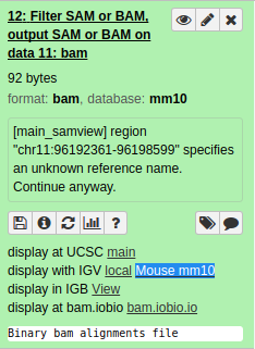Expand dataset and click highlighted link (on Linux systems you may need to install IGV separately and use local link).
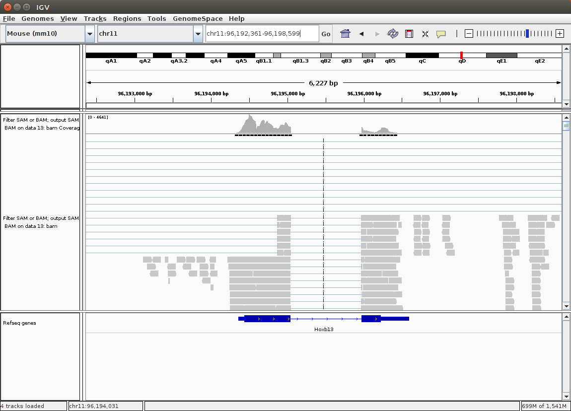Once IGV starts, focus it on the gene of interest by typing its name into the location box (in the image above the location box is on top of IGV interface and has coordinates chr11:96,192,361-96,198,599 in it) . In this case the gene is Hoxb13.
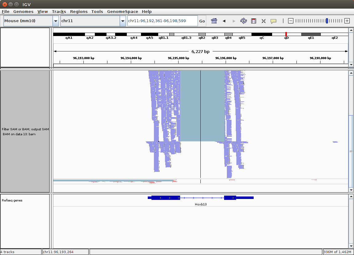Right click on the lift side of interface to (1) color, group, and sort alignments by first-of-pair strand and (2) set view to collapsed.

In the picture above you will see that the absolute majority of read pairs have their first read mapping on the negative strand (they are blue). At the same time the gene in the picture, Hoxb13, is on the positive strand (its arrows point from left to right). This this is a stranded RNA seq data were first cDNA strand is being sequenced. This implies that when we start actual analysis of this data we will use First Strand (R/RF) setting of HISAT.

Preparing dataset collections

Now we know that we are dealing with a stranded RNAseq experiment and that it may benefit from trimming the reads. Let's begin actual analysis. Instead of running a single tool multiple times on all your data, would you rather run a single tool on multiple datasets at once? To do this we will use dataset collections feature of Galaxy!

Copy datasets to a new history

We want to create a new clean history by moving the original sequence data. To do this we click on the cog () above the history pane and choose copy datasets and follow the instructions in the figure below:

A. Click on the cog () Choose "Copy Datasets" option:	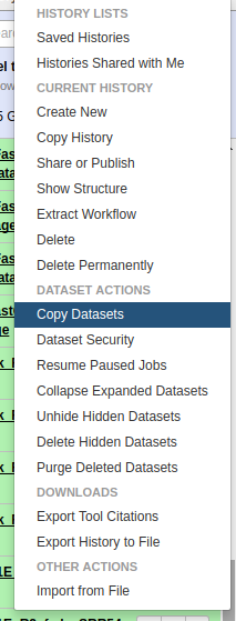B. Choose which datasets you need to copy: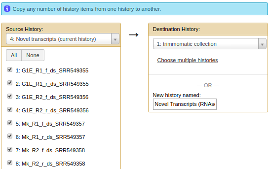 C. Click on the name of the newly created history:
Copying datasets into a new history	A: Use history options dropdown. B: Select datasets to copy and type a new for the new history (Novel Transcripts (RNAseq) in this case). C: Go to the new history by clicking on the link with its name.

Once all datasets are copied it will look something like this:

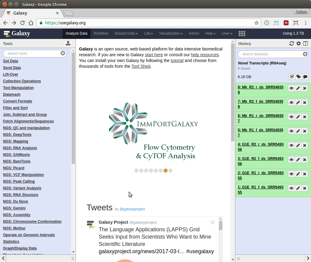New history with copied datasets

Create two dataset collections

We will create two dataset collections: one containing data for G1E cells and the other for megakaryocytes (you may want to review features of Galaxy's history system explained in this tutorial):

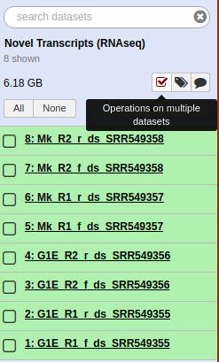
Make history items selectable by clicking checkbox () icon. This will allow individual datasets to be selected.|

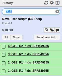
Show only G1E data by typing G1E in the search box.

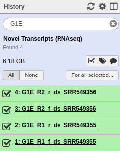
Select all shown datasets by clicking All.

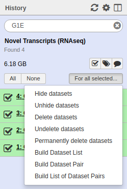
Use For all selected dropdown and select option Build List of Dataset Pairs to start collection builder.

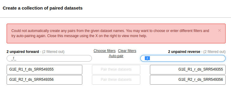
In the collection builder enter _f_ and _r_ in the two search boxes. Because datasets in out history are named as, for example, G1E_R1_f_ds_SRR549355, the _f_ and _r_ diffrentiate forward and reverse reads. Click Pair these datasets button.

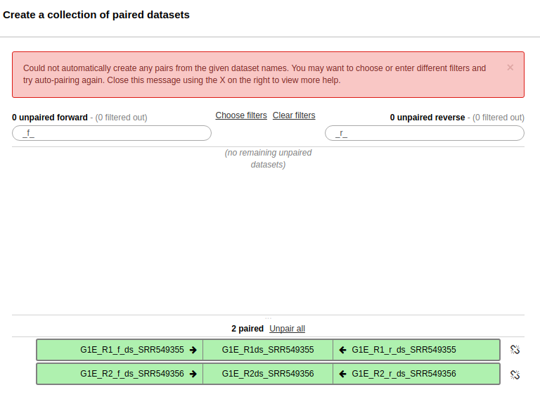
Datasets will become paired.

Scroll down, name the collection G1E and click Create list.

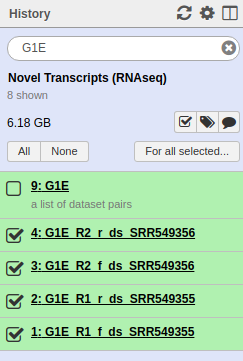
You will get a new item in the history representing that collectio.n

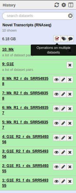
Repeat these steps for Megakarycytes datasets and you should get a history that looks like the one above.

Pre-processing, mapping, and post-processing

Here we will trim all reads in our dataset, map them, and filter mapped data.

Pre-processing: Trimming all datasets

Now that we have collections let's use Trimmomatic to trim all datasets in our analysis at once. We can do this directly on collections:

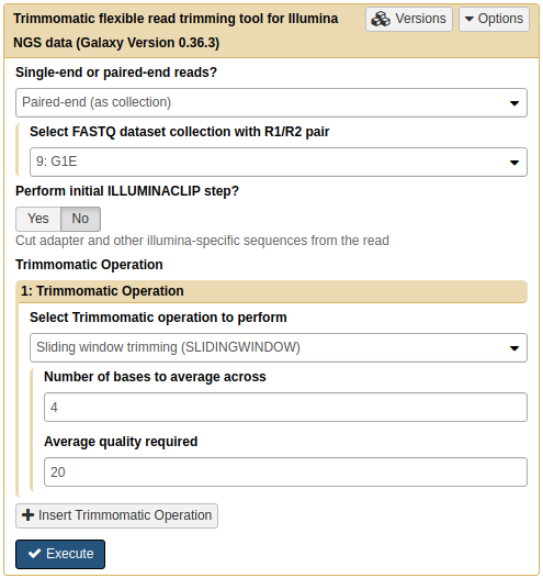Trimming an entire collection. Note that Single-end or paired-end reads? is set to Paired-end (as collection). This allows select collections (such G1E) as inputs.

This should be repeated for Mk collection as well (do it on your own). Note that Trimmomatic produces two output collection: one contained paired reads (labeled as paired; the one we want) and the one containing singletons (labeled as unpaired; the one we do not want in this case). We can simply delete collections that have unpaired in their names. It will be easier down the line if we rename collections to make easier to identify as analysis is progressing (collection tagging, which is currently in development, will alleviate this need in the near future). To rename a collection:

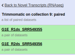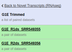Click on collection to see this interface	Simply edit its name (from Trimmomatic on collection... to G1E Trimmed and hit Enter

To make sense of the reads, their positions within mouse genome must be determined. This process is known as aligning or 'mapping' the reads to the reference genome. In the case of a eukaryotic transcriptome, most reads originate from processed mRNAs lacking introns. Therefore, they cannot be simply mapped back to the genome as we normally do for reads derived from DNA sequences. Instead, the reads must be separated into two categories:

• Reads contained within mature exons - these align perfectly to the reference genome
• Reads that span splice junctions in the mature mRNA - these align with gaps to the reference genome

Spliced mappers have been developed to efficiently map transcript-derived reads against genomes. HISAT is an accurate and fast tool for mapping spliced reads to a genome. Another popular spliced aligner is TopHat, but we will be using HISAT in this tutorial. For more details on these tools see our introductory RNAseq tutorial.

Spliced mapping with HISAT

We will run HISAT with the following settings:

• Single end or paired reads?: Collection of paired reads
• Source for the reference genome to align against: Use a built-in genome > Mouse (Mus Musculus): mm10
• Spliced alignment parameters: Specify spliced alignment parameters
• Specify strand-specific information: First Strand (R/RF)
• Transcriptome assembly reporting: Report alignments tailored for transcript assemblers including StringTie.

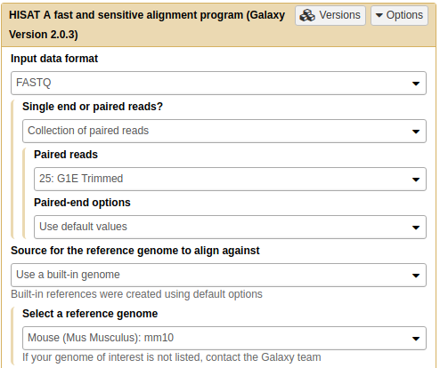HISAT settings. Upper part of HISAT interface showing that it is being run on a collection G1E against mm10 genome build. Do not forget to scroll down and set Spliced alignment parameters as explained above.

Post-processing: cleaning the BAM

After reads have been mapped it would make sense to restrict mapped reads to those than map in correct pairs and do not map to multiple locations. This can be done with SAMools -> Filter SAM or BAM tool:

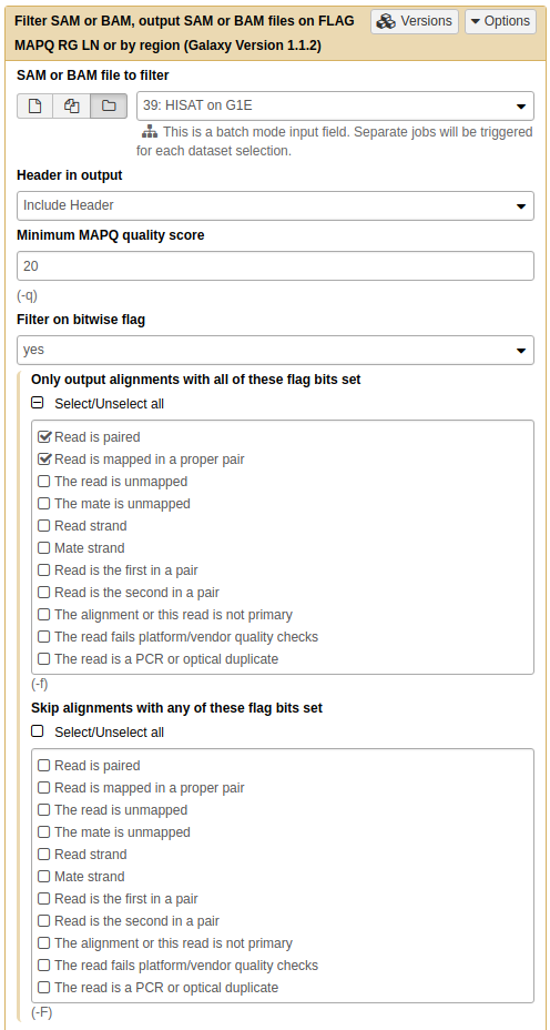|BAMTools Filter. Here we are filtering results of HISAT run (a dataset collection called HISAT on G1E) by retaining only reads with high mapping quality that are paired and mapped in a proper pair.

We will again rename collections to HISAT on G1E filtered and HISAT on Mk filtered:

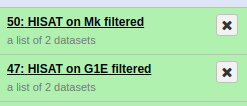HISAT results after filtering. Keeping names clear is important for smooth sailing!

De novo transcript reconstruction

Assembling transcripts in individual sampled with Stringtie

Now that we have mapped our reads to the mouse genome with HISAT, we want to determine transcript structures that are represented by the aligned reads. This is called de novo transcriptome reconstruction. This unbiased approach permits the comprehensive identification of all transcripts present in a sample, including annotated genes, novel isoforms of annotated genes, and novel genes. While common gene/transcript databases are quite large, they are not comprehensive, and the de novo transcriptome reconstruction approach ensures complete transcriptome(s) identification from the experimental samples. The leading tool for transcript reconstruction is Stringtie. Here, we will use Stringtie to predict transcript structures based on the reads aligned by HISAT and filtered as described above:

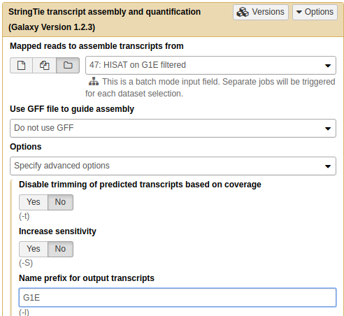|Running Stringtie on filtered mapped reads. Here it is run on collection G1E and we set Name prefix for output transcripts to G1E. When running Stringtie on collection Mk set this accordingly.

Stringtie generates assembled transcripts in GFF format. Below is an example of its output:

chr1 StringTie transcript 160938184 160940158 1000 + . gene_id "G1E.1"; transcript_id "G1E.1.1"; cov "12.347418"; FPKM "18.040417"; TPM "25.133554";
chr1 StringTie exon       160938184 160938232 1000 + . gene_id "G1E.1"; transcript_id "G1E.1.1"; exon_number "1"; cov "7.510204";

for description of fields in this dataset see Stringtie manual.

Creating unified transcriptome assembly

We just generated four transcriptomes with Stringtie representing each of the four RNA-seq libraries we are analyzing. Since these were generated in the absence of a reference transcriptome, and we ultimately would like to know what transcript structure corresponds to which annotated transcript (if any), we have to make a transcriptome database. We will use the tool Stringtie merge to combine redundant transcript structures across the four samples, provide non-redundant identifiers, and with the help of a reference annotation file annotate the nature/origin of each transcript (reference, novel isoform, intergenic transcript, antisense, etc.).

However, since we have ran Stringtie on each collection (G1E and Mk) independently it, in turn, has produced two collections each containing transcript assemblies for each replicate. Before we run Strigtie merge we need to merge the collections. This is done using Collection Operations -> Merge Collections tool:

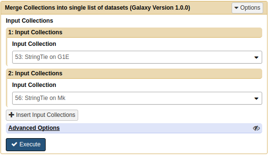Merging collection into a single collection. This assumes that you have renamed collections produced by Stringtie as Stringtie on G1E and Stringtie on Mk.

Now that the two collections are merged we will rename resulting collection Transcriptome. We are almost ready to run Stringtie merge on it. But in order to distinguish between novel and existing transcripts we will need provide Stringtie merge with a list of known annotated transcripts. For mouse genome version used in this tutorial (mm10) such a list can be downloaded from a Galaxy Library as was described above. Now we can finally run Stringtie merge:

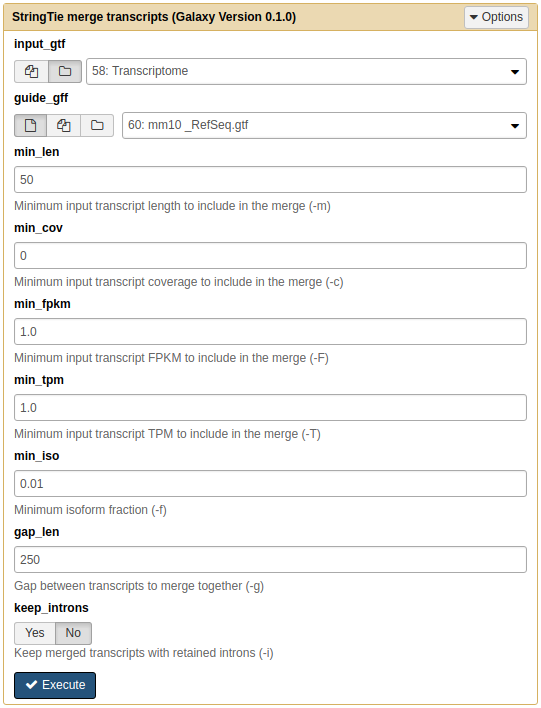Merging transcripts from G1E and Mk replicates into a single unified GFF dataset.

We will rename output of Stringtie merge as Merged transcriptome.

Analysis of the differential gene expression

We just generated a transcriptome database (a GFF output of Stringtie merge) that represents the transcripts present in the G1E and megakaryocytes samples. This database provides the location of our transcripts with non-redundant identifiers, as well as information regarding the origin of the transcript.

We now want to identify which transcripts are differentially expressed between the G1E and megakaryocyte cellular states. To do this we will implement a counting approach using FeatureCounts to count reads per transcript. Then we will provide this information to DESeq2 to generate normalized transcript counts (abundance estimates) and significance testing for differential expression.

Count the number of reads per transcript

To compare the abundance of transcripts between different cellular states, the first essential step is to quantify the number of reads per transcript. FeatureCounts is one of the most popular tools for counting reads in genomic features. In our case, we'll be using NGS: RNA Analysis -> FeatureCounts to count reads aligning in exons of our Stringtie merge generated transcriptome database.

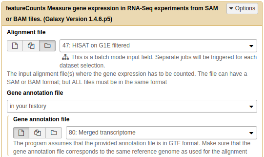Set input collection. In this case this is filtered HISAT output for G1E replicates (You will have to repeat featureCount calculation on Mk collection as well.)
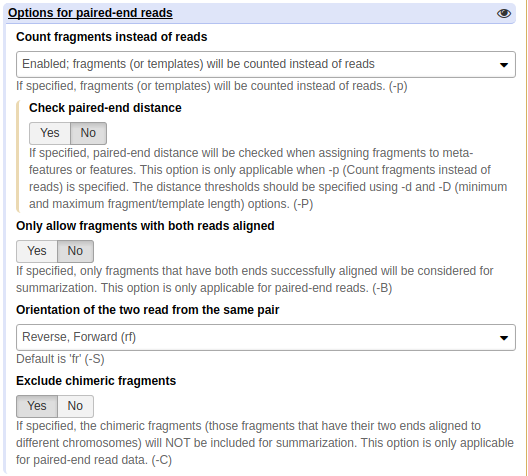Expand Options for paired-end reads, enable Count fragments instead of reads and set Orientation of the two read from the same pair to Reverse, Forward (rf).
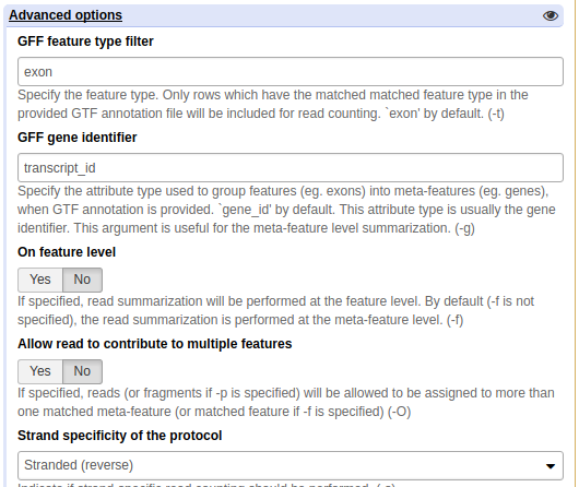Finally expand Advanced options, set GFF gene identifier to transcript_id, Strand specificity of the protocol to Stranded (reverse) and hit Enter.

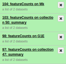Rename collection generated by featureCount as featureCounts on G1E and featureCounts on Mk.

Perform differential gene expression testing

Transcript expression is estimated from read counts, and attempts are made to correct for variability in measurements using replicates. This is absolutely essential to obtaining accurate results. We recommend having at least two biological replicates (although you should really have three or even more).

DESeq2 is a proven and widely used tool for differential gene expression analysis. It takes read counts produced by FeatureCounts and applies size factor normalization:

• Computation for each gene of the geometric mean of read counts across all samples
• Division of every gene count by the geometric mean
• Use of the median of these ratios as sample's size factor for normalization

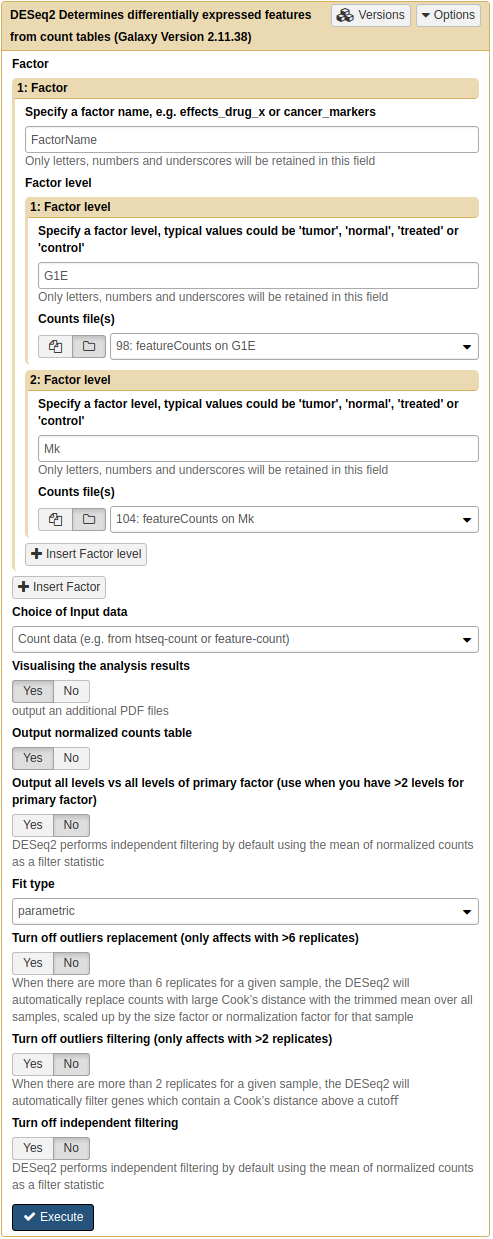|Running DeSeq2 on G1E and Mk counts. Note how Factor Levels are set. Output normalized counts table parameter is set to Yes.

The first output of DESeq2 is a tabular file. That looks like this (only three decimal points are shown):

1            2       3        4     5      6         7
--------------------------------------------------------------
MSTRG.977.1  697.447 -10.030  1.062 -9.444 3.583e-21 1.974e-18
MSTRG.78.1   645.022  10.656  1.195  8.915 4.873e-19 1.342e-16
MSTRG.129.1  368.102  -8.846  1.055 -8.379 5.328e-17 9.787e-15
MSTRG.1498.1 252.670   6.152  0.815  7.544 4.556e-14 6.277e-12
MSTRG.1434.1 372.478   4.855  0.666  7.288 3.125e-13 3.444e-11
NM_133804    257.129 -10.262  1.509 -6.798 1.060e-11 9.737e-10

where:

1. Gene identifiers
2. Mean normalized counts, averaged over all samples from both conditions
3. log₂ of the fold change (the values correspond to up- or downregulation relative to the condition listed as Factor level 1)
4. Standard error estimate for the log2 fold change estimate
5. Wald statistic
6. p-value for the statistical significance of this change
7. p-value adjusted for multiple testing with the Benjamini-Hochberg procedure which controls false discovery rate (FDR)

Making sense of the results

The output of DeSeq2 contain over 35,000 rows. Let's select transcripts with the most significant expression differences. For this we will filter DeSeq2 output on adjusted p-value using Filter and Sort -> Filter tool:

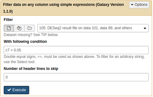Filtering to retain only genes with adjusted p-value above 0.05.

This retains 128 transcripts. You can see that in some cases log₂ fold change is positive and in some cases it is negative. To give you an idea on what this means let's look at normalized counts for genes with negative and positive change. One way to do this is to join the dataset we have just generated with Filter tool with normalized counts generated by DeSeq2. For this we will use Join, Subtract and Group -> Join two Datasets tool:

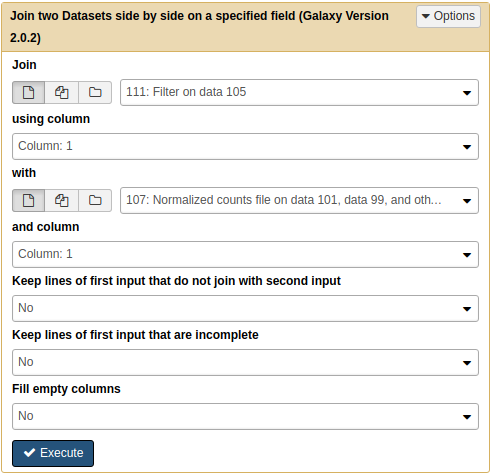Joining filtered DeSeq2 output with normalized counts.

Let's look at two first entries:

Last four columns are normalized counts for:                    Mk_1     Mk_2     G1E_1    G1E_2
--------------------------------------------------------------------------------------------------
MSTRG.977.1  697.447 -10.030  1.062 -9.444 3.583e-21 1.974e-18  2081.714 706.074    1.665    0.333
MSTRG.78.1   645.022  10.656  1.195  8.915 4.873e-19 1.342e-160    0.000   0.000 1311.325 1268.763

The last four columns are normalized reads counts for two megakarycyte and two G1E replicates, respectively. You can see that for MSTRG.977.1 log₂ fold change is -10.030 and there are practically no G1E reads. Conversely, in the case of MSTRG.78.1 log₂ fold change is 10.656 and there are no megakaryocyte reads. This is this case because we set G1E as the Factor level 1 while running DeSeq2 and positive change implies downregulation in megakaryocytes compared to G1E cells and vice versa. So to find all genes upregulated in Mk, for example, one would need to filter DeSeq2 output for fold change below 0.

In addition to the list of genes, DESeq2 outputs a graphical summary of the results, useful to evaluate the quality of the experiment:

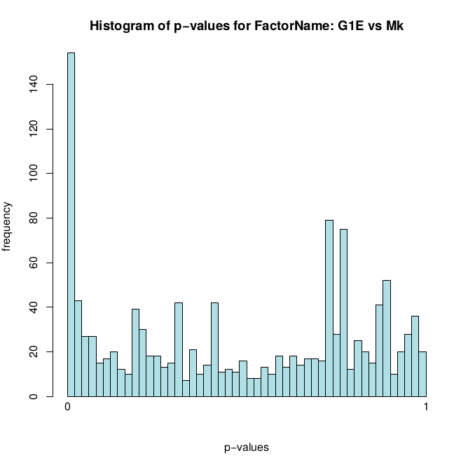Histogram of p-values for all tests.
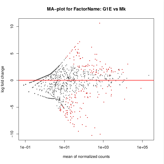MA plot: global view of the relationship between the expression change of conditions (log ratios, M), the average expression strength of the genes (average mean, A), and the ability of the algorithm to detect differential gene expression. The genes that passed the significance threshold (adjusted p-value < 0.1) are colored in red.
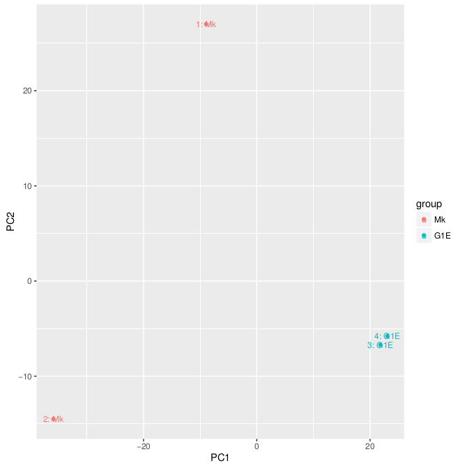Principal Component Analysis (PCA) and the first two axes. Each replicate is plotted as an individual data point. This type of plot is useful for visualizing the overall effect of experimental covariates and batch effects.
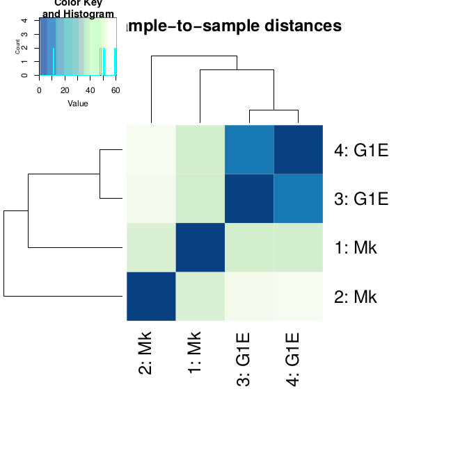Heatmap of sample-to-sample distance matrix: overview over similarities and dissimilarities between samples.
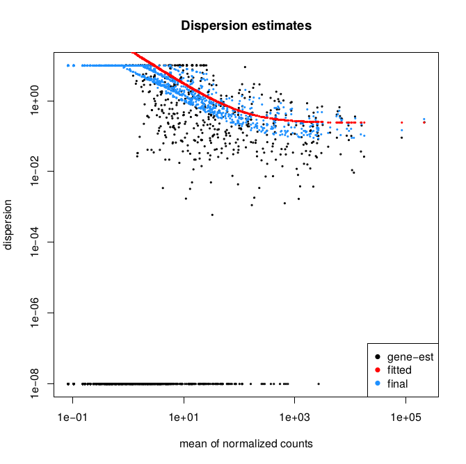Dispersion estimates: gene-wise estimates (black), the fitted values (red), and the final maximum a posteriori estimates used in testing (blue). This dispersion plot is typical, with the final estimates shrunk from the gene-wise estimates towards the fitted estimates. Some gene-wise estimates are flagged as outliers and not shrunk towards the fitted value. The amount of shrinkage can be more or less than seen here, depending on the sample size, the number of coefficients, the row mean and the variability of the gene-wise estimates.

For more information about DESeq2 and its outputs, you can have a look at DESeq2 documentation.

Visualization

Now that we have a list of transcript expression levels and their differential expression levels, it is time to visually inspect our transcript structures and the reads they were predicted from. It is a good practice to visually inspect (and present) loci with transcripts of interest. As we've seen above, Galaxy integrates well with the IGV browser.

Prepare BAM files

When looking at results it will helpful to see read coverage at the regions of interest. But we have four datasets corresponding to four replicates and in your own experiment there may be even more datasets. So let's first merge all HISAT BAM outputs into a single BAM file. However, to keep the relationship between individual reads and samples we need to add readgroup tags to each BAM file before merging. For this we will use a combination of tools:

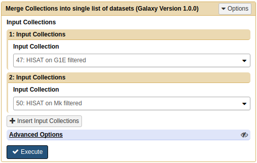First, merge filtered HISAT outputs into a single collection. This is done using Collection Operations -> Merge Collections tool. Rename this collection HISAT merged.
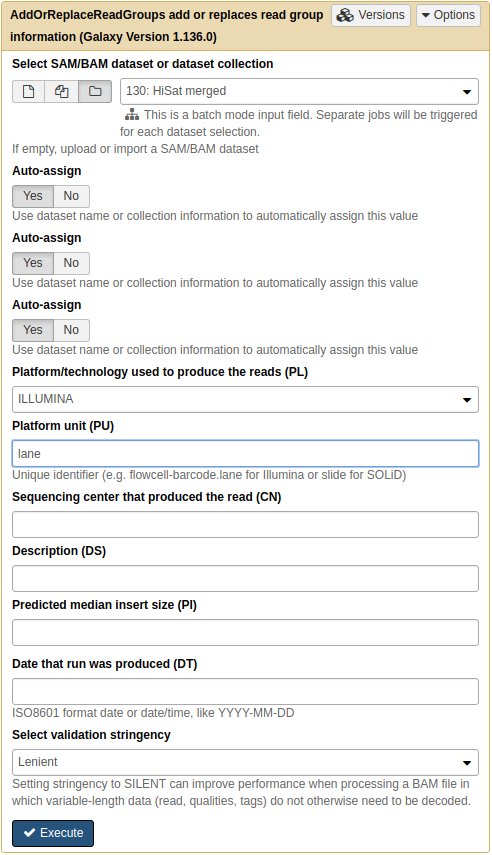Second, use NGS: Picard -> AddOrReplaceReadGroup to add readgroups as shown above. This will automatically set readgroups based on dataset names.
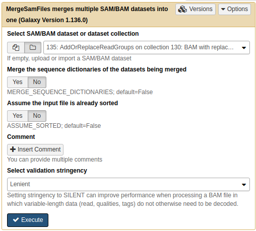Finally, use NGS: Picard -> MergeSamFiles to collapse the entire collection you've just produced at the previous step into a single BAM dataset. Name this dataset HISAT single BAM. We will use this dataset for visualization.

Starting and using IGV

To start IGV expand the merged dataset we have just generated:

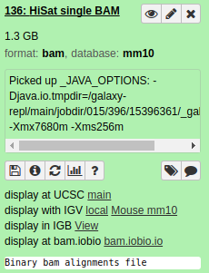Click on Mouse mm10 link (on Linux systems you may need to install IGV separately and use local link). This action will download and start IGV.

After IGV has started we will add to GTF files containing merged transcripts (the one produced here):

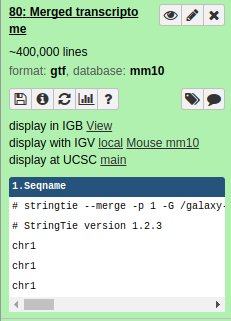|To display GFF with merged transcripts click on local IGV link.

Finally, direct IGV to the locus of interest by typing MSTRG.78.1 in the IGV's location box. MSTRG.78.1 is novel transcript which significantly overexpressed in G1E according to our DeSeq2 analysis:

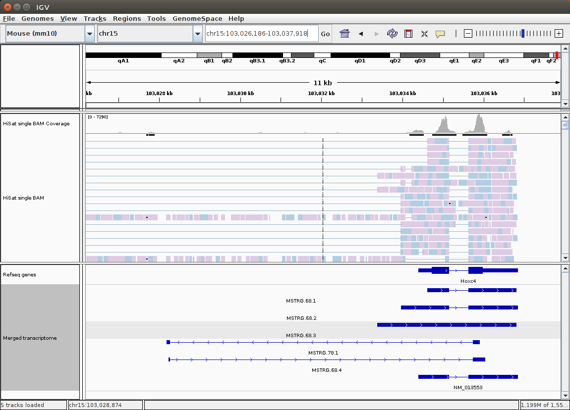|IGV view of the MSTRG.78.1 locus. |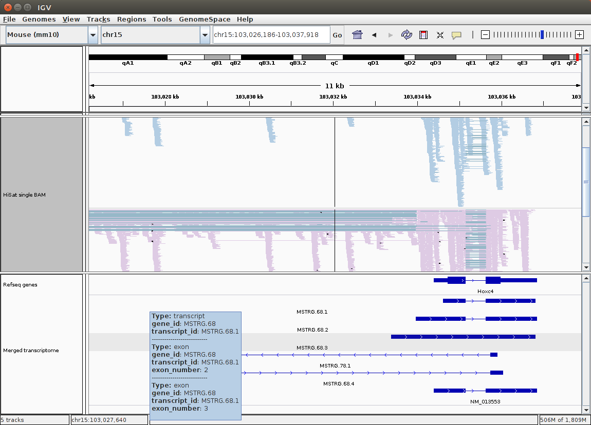| |Grouping and coloring alignments by readgroup will show that only G1E replicates contain any read data.

Conclusion

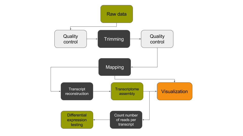
In this tutorial, we have analyzed real RNA sequencing data to extract useful information, such as which genes are up- or down-regulated by depletion of the Pasilla gene and which genes are regulated by the Pasilla gene. To answer these questions, we analyzed RNA sequence datasets using a reference-based RNA-seq data analysis approach. This approach can be sum up with the following scheme: